Fast Running Covariance Computation

Computes running covariance between time-series x and short-time pattern y.

RunningCov(x, y, circular = FALSE)

Arguments

x	A numeric vector.
y	A numeric vector, of equal or shorter length than x.
circular	Logical; whether running variance is computed assuming circular nature of x time-series (see Details).

Value

A numeric vector.

Details

Computes running covariance between time-series x and short-time pattern y.

The length of output vector equals the length of x. Parameter circular determines whether x time-series is assumed to have a circular nature. Assume \(l_x\) is the length of time-series x, \(l_y\) is the length of short-time pattern y.

If circular equals TRUE then

• first element of the output vector corresponds to sample covariance between x[1:l_y] and y,

• last element of the output vector corresponds to sample covariance between c(x[l_x], x[1:(l_y - 1)]) and y.

If circular equals FALSE then

• first element of the output vector corresponds to sample covariance between x[1:l_y] and y,

• the \(l_x - W + 1\)-th last element of the output vector corresponds to sample covariance between x[(l_x - l_y + 1):l_x],

• last W-1 elements of the output vector are filled with NA.

See runstats.demo(func.name = "RunningCov") for a detailed presentation.

Examples

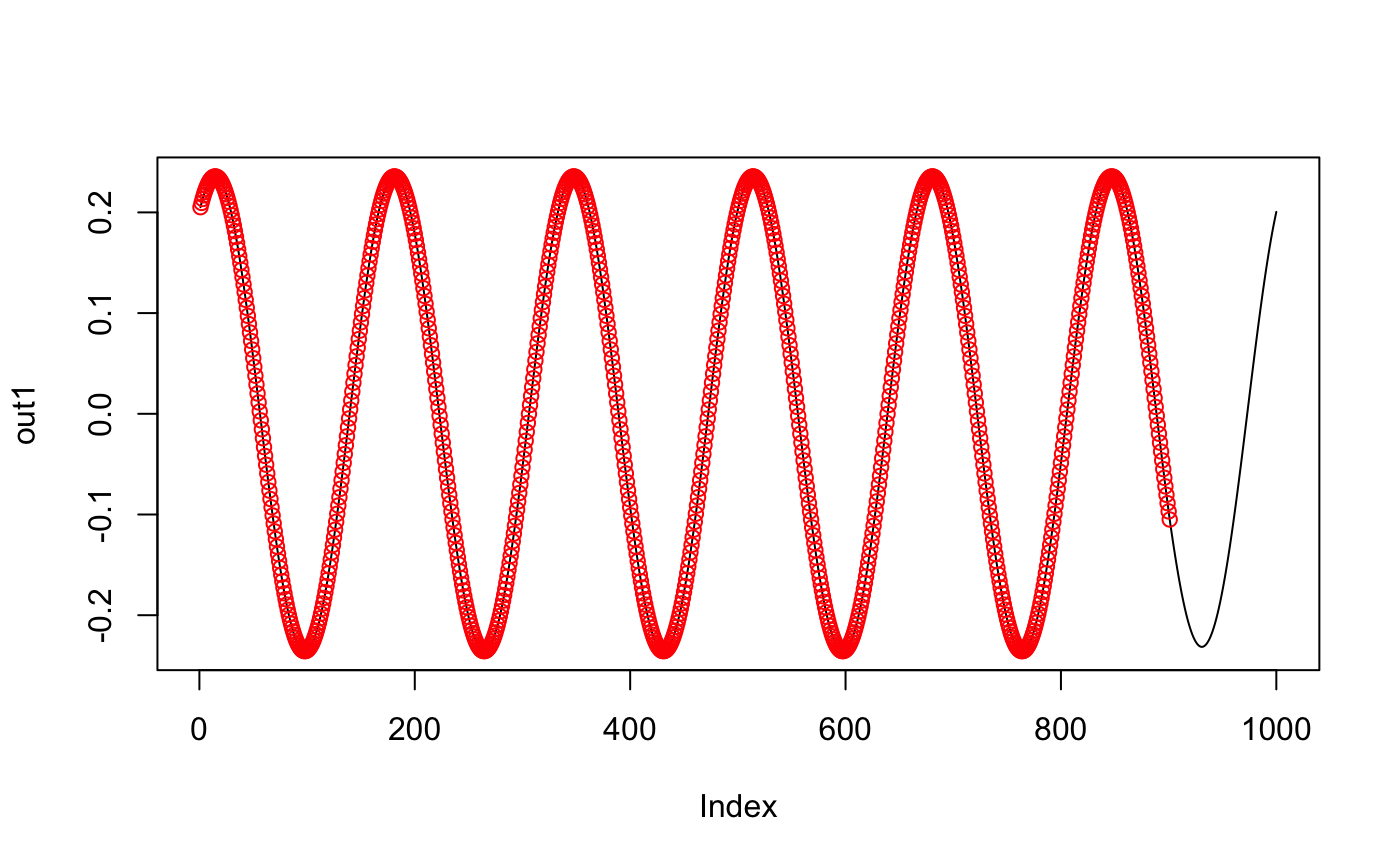
x <- sin(seq(0, 1, length.out = 1000) * 2 * pi * 6)
y <- x[1:100]
out1 <- RunningCov(x, y, circular = TRUE)
out2 <- RunningCov(x, y, circular = FALSE)
plot(out1, type = "l"); points(out2, col = "red")