Computing minute-level summary measures of physical activity from raw accelerometry data in R: AC, MIMS, ENMO, MAD, and AI

Jul 10, 2021 12 min read

In this post, we:

use dataset “Labeled raw accelerometry data captured during walking, stair climbing and driving” that is freely available on PhysioNet;
derive four minute-level summary measures of physical activity – AC, MIMS, ENMO, MAD, AI – from raw accelerometry data using SummarizedActigraphy R package;
summarize minute-level summary measures across walking and driving activities.

Table of Contents

Dataset “Labeled raw accelerometry data”

The dataset contains raw accelerometry data collected during outdoor walking, stair climbing, and driving for n=32 healthy adults. It is freely is available to download on PhysioNet at: https://doi.org/10.13026/51h0-a262

The study was led by Dr. Jaroslaw Harezlak, assisted by Drs. William Fadel and Jacek Urbanek.
Accelerometry data were collected simultaneously at four body locations: left wrist, left hip, left ankle, and right ankle, at a sampling frequency of 100 Hz.
The 3-axial ActiGraph GT3X+ devices were used to collect the data.
The data include labels of activity type performed for each time point of data collection (1=walking; 2=descending stairs; 3=ascending stairs; 4=driving; 77=clapping; 99=non-study activity).

We downloaded the data zip from PhysioNet and unpacked. This can be done manually from the website, or using download the data programmatically.

(Click to see the code to download the data.)

url <- paste0(
  "https://physionet.org/static/published-projects",
  "/accelerometry-walk-climb-drive",
  "/labeled-raw-accelerometry-data-captured-during-walking-stair-climbing-and-driving-1.0.0.zip")
destfile <- paste0(
  "/Users/martakaras/Downloads",
  "/labeled-raw-accelerometry-data-captured-during-walking-stair-climbing-and-driving-1.0.0.zip")
# download zip
result <- curl::curl_download(url, destfile = destfile, quiet = FALSE)
# unzip zip 
unzip(zipfile = destfile, exdir = dirname(destfile))

First, let’s look at raw accelerometry data of a single subject.

(Click to see the code.)

library(tidyverse)
library(lubridate)
library(lme4)
library(knitr)
# remotes::install_github("muschellij2/SummarizedActigraphy")
library(SummarizedActigraphy)
library(MIMSunit)
library(activityCounts)
options(digits.secs = 3)
options(scipen=999)

# define path to raw data files directory
raw_files_dir <- paste0(
  "/Users/martakaras/Downloads",
  "/labeled-raw-accelerometry-data-captured-during-walking-stair-climbing-and-driving-1.0.0",
  "/raw_accelerometry_data")

# single participant's raw accelerometry data
dat_fpaths <- list.files(raw_files_dir, full.names = TRUE)
dat_i <- read_csv(dat_fpaths[1])

dat_i

# A tibble: 303,300 x 14
   activity time_s   lw_x   lw_y   lw_z   lh_x   lh_y   lh_z   la_x  la_y   la_z
      <dbl>  <dbl>  <dbl>  <dbl>  <dbl>  <dbl>  <dbl>  <dbl>  <dbl> <dbl>  <dbl>
 1       99   0.01  0.039  1.02  -0.02  -0.18   1.23   0.023  0.156 0.855 -0.582
 2       99   0.02 -0.629 -0.461  0.973 -0.246  0.137  0.969 -0.707 0.559  0.449
 3       99   0.03 -0.926 -1.26   0.691  0.238 -0.328  1.22  -1.44  1.37   0.367
 4       99   0.04 -0.871 -1.50  -0.246  0.711 -0.484  0.414 -1.66  1.64  -0.543
 5       99   0.05 -0.727 -1.62  -0.559  1.03  -0.297  0.145 -1.76  1.68  -0.918
 6       99   0.06 -0.543 -1.66  -0.629  1.12  -0.246  0.137 -1.80  1.65  -0.988
 7       99   0.07 -0.348 -1.64  -0.609  1.24  -0.426  0.047 -1.76  1.57  -0.992
 8       99   0.08 -0.16  -1.60  -0.566  1.18  -0.539 -0.008 -1.63  1.53  -1.02 
 9       99   0.09 -0.012 -1.53  -0.523  1.03  -0.633 -0.043 -1.13  1.87  -0.738
10       99   0.1   0.117 -1.43  -0.484  0.922 -0.766 -0.047  0.285 1.37  -0.156
# … with 303,290 more rows, and 3 more variables: ra_x <dbl>, ra_y <dbl>,
#   ra_z <dbl>

Each file contains 14 variables:

activity – type of activity (1=walking; 2=descending stairs; 3=ascending stairs; 4=driving; 77=clapping; 99=non-study activity);
time_s – time from device initiation (seconds [s]);
lw_x, lw_y, lw_z – acceleration [g] measured by a left wrist-worn sensor at axis x, y, z;
lh_x, lh_y, lh_z – acceleration [g] measured by a left hip-worn sensor at axis x, y, z;
la_x, la_y, la_z – acceleration [g] measured by a left ankle-worn sensor at axis x, y, z;
ra_x, ra_y, ra_z – acceleration [g] measured by a right ankle-worn sensor at axis x, y, z.

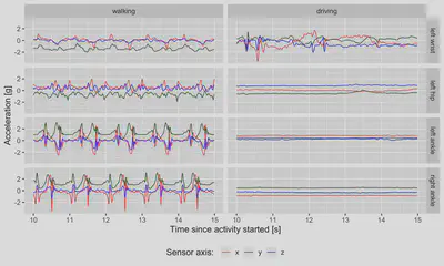
An exemplary few seconds of raw data from of walking and driving activities, collected by sensors at four different locations:

(Click to see the code.)

loc_id_levels <- c("lw", "lh", "la", "ra")
loc_id_labels <- c("left wrist", "left hip", "left ankle", "right ankle")
activity_levels <- c("walking", "driving")
plt_df <- 
  dat_i %>%
  filter(activity %in% c(1,4)) %>%
  group_by(activity) %>%
  mutate(time_s = time_s - min(time_s)) %>%
  ungroup() %>%
  filter(time_s >= (5 + 5), time_s < (5 + 10)) %>%
  mutate(activity = recode(activity, '1' = 'walking', '4' = 'driving')) %>%
  pivot_longer(cols = -c(activity, time_s)) %>%
  separate(name, c("loc_id", "axis_id"), sep = "_") %>%
  mutate(activity = factor(activity, levels = activity_levels)) %>%
  mutate(loc_id = factor(loc_id, levels = loc_id_levels, labels = loc_id_labels)) 
plt_raw_data <- 
  ggplot(plt_df, aes(x = time_s, y = value, color = axis_id)) + 
  geom_line() + 
  facet_grid(loc_id ~ activity) + 
  scale_y_continuous(limits = c(-1, 1) * max(abs(plt_df$value))) + 
  labs(y = "Acceleration [g]",
       x = "Time since activity started [s]",
       color = "Sensor axis: ") + 
  theme_gray(base_size = 14) + 
  theme(legend.position="bottom") + 
  scale_color_manual(values = c("red", "darkgreen", "blue"))

plt_raw_data

Computing minute-level summary measures of raw accelerometry data

Summary measures

A number of open-source measures have been proposed to aggregate subsecond-level accelerometry data. These include:

Monitor Independent Movement Summary (MIMS) (John et al., 2019),
Euclidean Norm Minus One (ENMO) (van Hees et al., 2013),
Mean Amplitude Deviation (MAD) (Vähä-Ypyä et al., 2015),
Activity Index (AI) (Bai et al., 2016).

In addition, attempts have been made to reverse-engineer proprietary activity counts (AC) generated by ActiLife software from data collected by ActiGraph accelerometers. These include:

activityCounts R package – allows generating “ActiLife counts from raw acceleration data for different accelerometer brands and it is developed based on the study done by Brond et al., 2017”.

SummarizedActigraphy R package

We derive the measures using SummarizedActigraphy R package. The package was authored by John Muschelli and is available on GitHub (link).

It uses some of the existing R software under the hood to compute some part of the measures:

MIMSunit R package to compute MIMS,
activityCounts R package to compute AC.

It computes some other measures straightfoward from their definition, e.g.: MAD, AI.

Note: the recommendations in the ENMO paper state data calibration preprocessing step. I observed an issue while attempting to run the calibration for files of less than 2h of duration which is the case for the exemplary data we use here. Therefore, here, we do not use data calibration. However, we successfully used SummarizedActigraphy R package to calibrate data and compute ENMO for hundreds of longer duration data files in the past – see this R script.

Preparing the data input

We use raw accelerometry data from a wrist-worn sensor.

(Click to see notes and code.)

Note:

SummarizedActigraphy R package needs data with observation timestamp in the form of POSIXct class. This timestamp column must be named HEADER_TIME_STAMP; the specific column naming is needed due to some issue reported for MIMSunit R package.
We hence create a “fake” POSIXct column named HEADER_TIME_STAMP.
The option options(digits.secs = 3) was used on the top of this R script to allow displaying decimal time part.

We first demonstrate the code for one participant.

dat_input_i <- 
  dat_i %>% 
  mutate(HEADER_TIME_STAMP = seq(from = ymd_hms("2021-01-01 00:00:00"), by = 0.01, length.out = nrow(dat_i))) %>%
  select(HEADER_TIME_STAMP, X = lw_x, Y = lw_y, Z = lw_z)

dat_input_i

# A tibble: 303,300 x 4
   HEADER_TIME_STAMP            X      Y      Z
   <dttm>                   <dbl>  <dbl>  <dbl>
 1 2021-01-01 00:00:00.000  0.039  1.02  -0.02 
 2 2021-01-01 00:00:00.009 -0.629 -0.461  0.973
 3 2021-01-01 00:00:00.019 -0.926 -1.26   0.691
 4 2021-01-01 00:00:00.029 -0.871 -1.50  -0.246
 5 2021-01-01 00:00:00.039 -0.727 -1.62  -0.559
 6 2021-01-01 00:00:00.049 -0.543 -1.66  -0.629
 7 2021-01-01 00:00:00.059 -0.348 -1.64  -0.609
 8 2021-01-01 00:00:00.069 -0.16  -1.60  -0.566
 9 2021-01-01 00:00:00.079 -0.012 -1.53  -0.523
10 2021-01-01 00:00:00.089  0.117 -1.43  -0.484
# … with 303,290 more rows

We use package’s helper function to check if sample rate is being determined correctly (should be 100 Hz).

get_sample_rate(dat_input_i)

[1] 100

Computing the measures

We calculate minute-level summary measures: AC, MIMS, ENMO, MAD, AI. The output shows values of the measures per each minute.

out_i = SummarizedActigraphy::calculate_measures(
  df = dat_input_i, 
  dynamic_range = c(-8, 8),  # dynamic range
  fix_zeros = FALSE,         # fixes zeros from idle sleep mode -- not needed in our case 
  calculate_mims = TRUE,     # uses algorithm from MIMSunit package
  calculate_ac = TRUE,       # uses algorithm from activityCounts package 
  flag_data = FALSE,         # runs raw data quality control flags algorithm -- not used in our case  
  verbose = FALSE)

======================================================================================

out_i <- out_i %>% select(HEADER_TIME_STAMP = time, AC, MIMS = MIMS_UNIT, ENMO = ENMO_t, MAD, AI)
out_i

# A tibble: 51 × 6
   HEADER_TIME_STAMP            AC  MIMS     ENMO     MAD    AI
   <dttm>                    <dbl> <dbl>    <dbl>   <dbl> <dbl>
 1 2021-01-01 00:00:00.000  3623.  19.3  0.0882   0.140    7.62
 2 2021-01-01 00:01:00.000  2460.  14.8  0.0544   0.0971   5.84
 3 2021-01-01 00:02:00.000   648.   6.52 0.00607  0.0192   2.44
 4 2021-01-01 00:03:00.000    36.2  1.86 0.000769 0.00862  1.03
 5 2021-01-01 00:04:00.000  8084.  34.8  0.323    0.316   15.1 
 6 2021-01-01 00:05:00.000 13845.  60.1  0.442    0.358   25.3 
 7 2021-01-01 00:06:00.000 10549.  44.1  0.475    0.248   18.7 
 8 2021-01-01 00:07:00.000 11219.  45.8  0.508    0.244   19.6 
 9 2021-01-01 00:08:00.000 11624.  51.6  0.393    0.338   22.1 
10 2021-01-01 00:09:00.000 11049.  45.8  0.404    0.288   20.0 
# … with 41 more rows

Next, we calculate the measures for all n=32 subjects.

(Click to see the code.)

out_all <- data.frame()
for (dat_fpath_i in dat_fpaths){ #  dat_fpath_i <- dat_fpaths[1]
  message(basename(dat_fpath_i))
  # read data 
  basename_i <- gsub(".csv", "", basename(dat_fpath_i))
  dat_i <- read.csv(dat_fpath_i) 
  # prepare data input
  ts_i <- seq(from = ymd_hms("2021-01-01 00:00:00"), by = 0.01, length.out = nrow(dat_i))
  dat_input_i <- 
    dat_i %>% 
    mutate(HEADER_TIME_STAMP = ts_i) %>%
    select(HEADER_TIME_STAMP, X = lw_x, Y = lw_y, Z = lw_z)
  # compute the measures 
  out_i = SummarizedActigraphy::calculate_measures(
    df = dat_input_i, 
    dynamic_range = c(-8, 8),  # dynamic range
    fix_zeros = FALSE,         # fixes zeros from idle sleep mode -- not needed in our case 
    calculate_mims = TRUE,     # uses algorithm from MIMSunit package
    calculate_ac = TRUE,       # uses algorithm from activityCounts package 
    flag_data = FALSE,         # runs raw data quality control flags algorithm -- not used in our case  
    verbose = FALSE)
  out_i <- out_i %>% select(HEADER_TIME_STAMP = time, AC, MIMS = MIMS_UNIT, MAD, AI)
  out_i <- mutate(out_i, subj_id = basename_i, .before = everything())
  # append subject-specific measures to all subjects file 
  out_all <- rbind(out_all, out_i)
}

Minute-level physical activity measures during walking and driving activities

Merging physical activity measures with physical activity labels

Next, we merge the minute-level physical-activity measures with the activity labels. We only keep the minutes for which all the measurements were labelled with no more than one type of activity.

(Click to see the code.)

labels_df_all <- data.frame()
for (dat_fpath_i in dat_fpaths){ #  dat_fpath_i <- dat_fpaths[1]
  message(basename(dat_fpath_i))
  # read data 
  basename_i <- gsub(".csv", "", basename(dat_fpath_i))
  dat_i <- read.csv(dat_fpath_i) 
  # aggregate activity labels
  ts_i <- seq(from = ymd_hms("2021-01-01 00:00:00"), by = 0.01, length.out = nrow(dat_i))
  labels_df_i <- 
    dat_i %>% 
    mutate(HEADER_TIME_STAMP = ts_i) %>%
    mutate(HEADER_TIME_STAMP = lubridate::floor_date(HEADER_TIME_STAMP, "1 min")) %>%
    group_by(HEADER_TIME_STAMP) %>%
    filter(n_distinct(activity) == 1) %>%
    filter(row_number() == 1) %>%
    # 1=walking; 2=descending stairs; 3=ascending stairs; 4=driving
    filter(activity %in% c(1,2,3,4)) %>%
    ungroup() %>%
    select(HEADER_TIME_STAMP, activity) 
  labels_df_i <- mutate(labels_df_i, subj_id = basename_i, .before = everything())
  # append subject-specific measures to all subjects file 
  labels_df_all <- rbind(labels_df_all, labels_df_i)
}
# recode activity label
labels_df_all <- labels_df_all %>%
  mutate(activity = recode(activity, '1' = 'walking', '2' = 'descending_stairs', 
                           '3' = 'ascending_stairs', '4' = 'driving'))

# merge: 
# (1) physical activity minute-level measures, 
# (2) physical activity minute-level activity labels
out_all_merged <- 
  out_all %>% 
  inner_join(labels_df_all, by = c("subj_id", "HEADER_TIME_STAMP"))

out_all_merged

# A tibble: 686 × 8
   subj_id    HEADER_TIME_STAMP           AC  MIMS   ENMO    MAD    AI activity
   <chr>      <dttm>                   <dbl> <dbl>  <dbl>  <dbl> <dbl> <chr>   
 1 id00b70b13 2021-01-01 00:06:00.000 10549. 44.1  0.475  0.248  18.7  walking 
 2 id00b70b13 2021-01-01 00:07:00.000 11219. 45.8  0.508  0.244  19.6  walking 
 3 id00b70b13 2021-01-01 00:11:00.000 11026. 42.3  0.498  0.215  18.9  walking 
 4 id00b70b13 2021-01-01 00:12:00.000 10561. 42.1  0.486  0.231  19.1  walking 
 5 id00b70b13 2021-01-01 00:13:00.000 13297. 53.9  0.591  0.325  23.1  walking 
 6 id00b70b13 2021-01-01 00:21:00.000  2603. 14.5  0.0501 0.0413  4.80 driving 
 7 id00b70b13 2021-01-01 00:23:00.000   499.  6.65 0.0534 0.0537  3.59 driving 
 8 id00b70b13 2021-01-01 00:24:00.000   398.  6.06 0.0537 0.0496  3.49 driving 
 9 id00b70b13 2021-01-01 00:25:00.000   130.  5.92 0.0542 0.0560  3.67 driving 
10 id00b70b13 2021-01-01 00:26:00.000   414.  7.00 0.0469 0.0561  3.55 driving 
# … with 676 more rows

table(out_all_merged$activity)


driving walking 
    569     117

Visualizing physical activity measures across activity types

We visualize values of minute-level physical activity measures. Note these only used data collected with a sensor located at left wrist.

(Click to see the code.)

name_levels <- c("AC", "MIMS", "ENMO",  "MAD", "AI")
activity_levels <- c("walking", "driving")
# define data subsets with one activity type only 
df_walk <- out_all_merged %>% filter(activity == "walking") 
df_driv <- out_all_merged %>% filter(activity == "driving")
# estimate sample population mean for each measure via LMM
measure_mean_vals <- c(
  # walking 
  fixef(lmer(AC ~ (1 | subj_id), data = df_walk))[1],
  fixef(lmer(MIMS ~ (1 | subj_id), data = df_walk))[1],
  fixef(lmer(ENMO ~ (1 | subj_id), data = df_walk))[1],
  fixef(lmer(MAD ~ (1 | subj_id), data = df_walk))[1],
  fixef(lmer(AI ~ (1 | subj_id), data = df_walk))[1],
   # driving 
  fixef(lmer(AC ~ (1 | subj_id), data = df_driv))[1],
  fixef(lmer(MIMS ~ (1 | subj_id), data = df_driv))[1],
  fixef(lmer(ENMO ~ (1 | subj_id), data = df_driv))[1],
  fixef(lmer(MAD ~ (1 | subj_id), data = df_driv))[1],
  fixef(lmer(AI ~ (1 | subj_id), data = df_driv))[1]
)
measure_mean_df <- data.frame(
  value = measure_mean_vals,
  name = rep(name_levels, times = 2),
  activity = rep(activity_levels, each = 5)
)
measure_mean_df_w <- 
  measure_mean_df %>%
  mutate(value = round(value, 2)) %>% 
  pivot_wider(names_from = activity)
# define subject-specific means 
out_all_l <- 
  out_all_merged %>%
  pivot_longer(cols = all_of(name_levels)) 
out_all_l_agg <- 
  out_all_l %>%
  group_by(subj_id, name, activity) %>%
  summarise(value = mean(value))
subj_id_levels <- 
  out_all_l_agg %>%
  filter(name == "AC", activity == "walking") %>%
  arrange(desc(value)) %>%
  pull(subj_id)
# mutate data frames used on the plot to have factors at certain levels order
measure_mean_df <- 
  measure_mean_df %>%
  mutate(activity = factor(activity, levels = activity_levels)) %>%
  mutate(name = factor(name, levels = name_levels))
out_all_l <- 
  out_all_l %>%
  mutate(subj_id = factor(subj_id, levels = subj_id_levels),
         activity = factor(activity, levels = activity_levels)) %>%
  mutate(name = factor(name, levels = name_levels))
out_all_l_agg <-
  out_all_l_agg %>%
   mutate(subj_id = factor(subj_id, levels = subj_id_levels),
         activity = factor(activity, levels = activity_levels)) %>%
  mutate(name = factor(name, levels = name_levels))

First, we estimated sample population mean for each minute-level measure via linear mixed model (LMM).

kable(measure_mean_df_w)

name	walking	driving
AC	7616.48	801.15
MIMS	34.86	7.10
ENMO	0.24	0.04
MAD	0.26	0.05
AI	15.01	3.31

Next, we plot minute-level physical activity measures:

individual measure values (red) for each subject,
mean measure value (black) for each subject,
sample population mean for each measure (dashed horizontal line) estimated via LMM.

On each plot panel, subject IDs (x-axis) are sorted by average AC during walking (left-top plot panel).

(Click to see the code.)

plt_measures <- 
  ggplot(out_all_l, 
         aes(x = subj_id, y = value)) + 
  geom_hline(data = measure_mean_df,
             aes(yintercept = value), 
             linetype = 2, size = 0.2) + 
  geom_point(size = 0.5, alpha = 0.3, color = "red") + 
  geom_point(data = out_all_l_agg, 
             aes(x = subj_id, y = value),
             size = 0.5, color = "black") + 
  facet_grid(name ~ activity, scales = "free") + 
  labs(x = "Subject ID", y = "") + 
  theme_gray(base_size = 14) +    
  theme(panel.grid.major = element_line(size = 0.3),  
        panel.grid.minor = element_blank(),
        axis.text.x = element_text(size = 6, angle = 90, vjust = 0.5, hjust = 1))

plt_measures

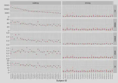
The above plot highlights what are minute-level summary measures of physical activity from raw accelerometry data: AC, MIMS, ENMO, MAD, and AI, across two different activities (walking, driving) in the study sample of n=32 healthy individuals.

Acknowledgements

I’d like to thank John Muschelli for feedback on this tutorial.

Citation info

Please cite SummarizedActigraphy R package, if applicable.

Please cite raw accelerometry dataset DOI, if applicable (go to see this dataset citation options).

Computing minute-level summary measures of physical activity from raw accelerometry data in R: AC, MIMS, ENMO, MAD, and AI

Dataset “Labeled raw accelerometry data”

Computing minute-level summary measures of raw accelerometry data

Summary measures

SummarizedActigraphy R package

Preparing the data input

Computing the measures

Minute-level physical activity measures during walking and driving activities

Merging physical activity measures with physical activity labels

Visualizing physical activity measures across activity types

Acknowledgements

Citation info

Marta Karas

Senior Manager, Statistics