Repeated Measures Correlation (rmcorr): when may be not an ideal choice to quantify the association
In this post, we use the Repeated Measures Correlation (rmcorr) approach to quantify association between two continuous measures recorded multiple times per study subject.
I recently learned about the rmcorr approach and explored it with a view of applying in one of the current projects. I think rmcorr is a very interesting method with neat interpretation. Here, I highlight key notes from how the rmcorr works, and I point to a few cases where I expect that rmcorr may be not an ideal choice to quantify the association.
Table of Contents
Repeated Measures Correlation
The Bakdash et al. (2017) paper Repeated Measures Correlation discusses within-participants correlation to analyze the common intra-individual association for paired repeated measures. The paper provides background information, methods description, R package reference, and discussion on tradeoffs with rmcorr as compared to multilevel modeling.
Method
In short, rmcorr:
- Is based on ANCOVA analysis: it considers a subject as a factor-level variable to remove between-person variation. ANCOVA model is set to estimate subjects’ common regression slope $\beta$.
- The rmcorr correlation coefficient is calculated using sums of squares for the Measure and for the error from the above ANCOVA model and its sign is determined by the sign (positive vs. negative) of estimated $\beta$.
- It has a nice, intuitive interpretation.
- Authors argue is “comparable to linear multilevel model (LMM) with random intercept only and a fixed effect”.
Key notes
Key notes on rmcorr:
- rmcorr does not allow for slope variation by subject,
- rmcorr does not utilize any of LMM’s partial-pooling idea (i.e., where for subjects with a relatively smaller number of observations, their estimates are “shrunk” closer to the overall population average);
and hence, as the authors noted, rmcorr may be not an ideal choice to quantify the association:
- when the effect slope varies between subjects.
I also thought having random slopes is even more problematic:
- when the number of observations varies between subjects (e.g., varies between 2-10),
- when there are influential observation(s) (e.g., subject(s) with wide $x$ values range).
Scenarios
To illustrate the above notes, 4x2 simple data scenarios are considered.
- In each scenario, data on N = 20 subjects with 2 continuous variables ($x$, $y$), recorded at multiple occasions for each subject, are simulated.
- The scenarios differ in true data-generating model that is assumed:
- Scenario 1: random intercept only;
- Scenario 2: random intercept and random slope (uncorrelated);
- Scenario 3: random intercept and random slope (uncorrelated), added one subject with influential observations;
- Scenario 4: random intercept and random slope (uncorrelated), unbalanced number of observations per subject.
- For each scenario, two versions are considered, assuming: (a): small variance of residual error; (b) large variance of residual error.
To show the results:
- For each scenario, 1 data set is used and results from applying 2 approaches are shown:
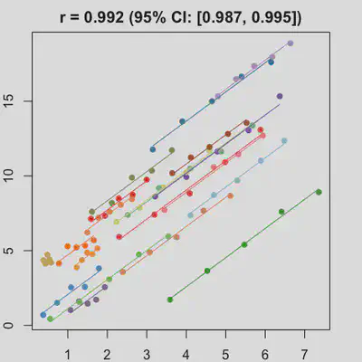
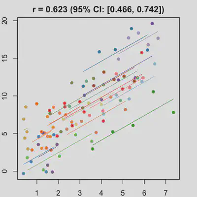
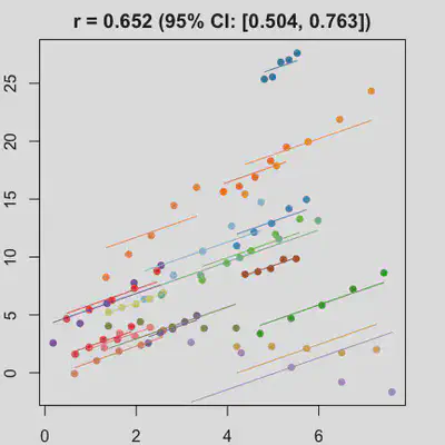
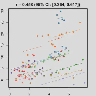
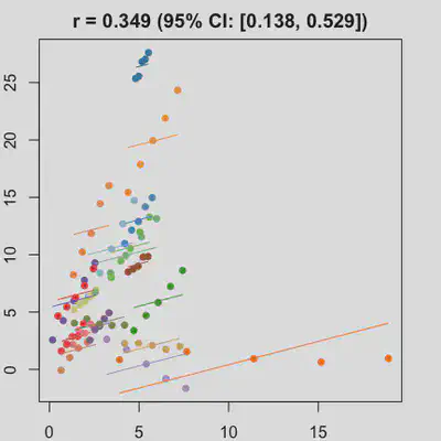
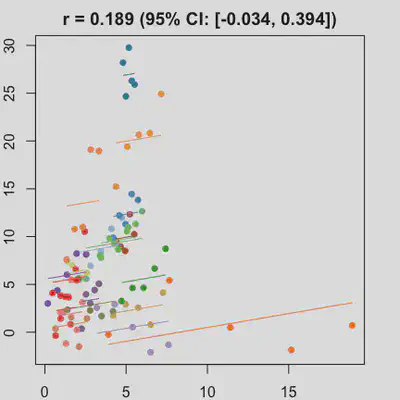
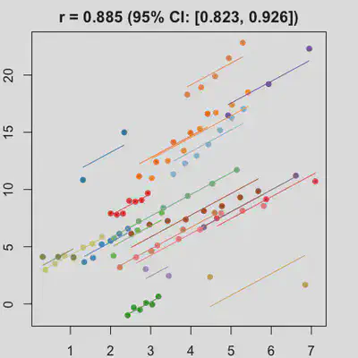
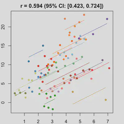
- left plot: rmcorr with an estimate of “repeated measures correlation”,
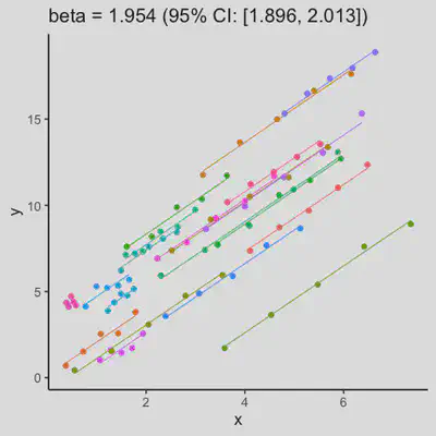
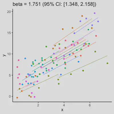
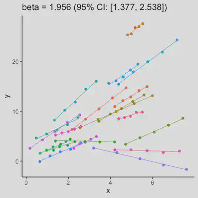
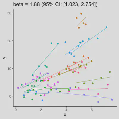
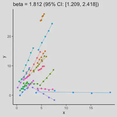
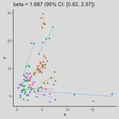
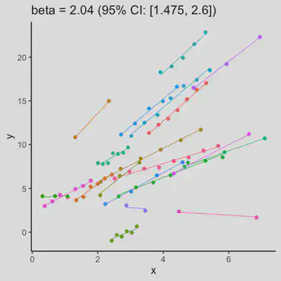
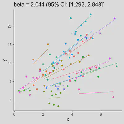
- right plot: LMM fit with an estimate of fixed effect slope.
- For all scenarios, left plot points same as right plot points (the same data used for 2 approaches).
- For all scenarios, population-level effect $x$ on $y$ was assumed to be equal $2.0$.
- For all scenarios, LMM assumes random intercept and random slope for $x$, and a fixed effect for $x$.
(Click to see R code shared for all simulations.)
library(tidyverse)
library(lme4)
library(lmerTest)
library(rmcorr)
library(MASS)

# define simulation parameters
# number of subjects
M <- 20
# number of repeated measures per subjects (for all except last two scenarios)
k <- 5

#' Function to apply two approaches to `dat` data set:
#' (1) rmcorr with an estimate of "repeated measures correlation",
#' (2) LMM fit with an estimate of fixed effect slope
est_and_plot <- function(dat){
  # approach 1
  rmcorr_out <- rmcorr(subj_id, x, y, dat)
  plt_label <- paste0("r = ", round(rmcorr_out$r, 3), " (95% CI: [", paste0(round(rmcorr_out$CI, 3), collapse = ", "), "])")
  par(mar = rep(2, 4))
  plot(rmcorr_out, main = plt_label)

  # approach 2
  lmm_out <- lmer(y ~ x + (1 + x | subj_id), data = dat)
  conf_est <- summary(lmm_out)$coef[2, 1]
  conf_out <- as.vector(confint(lmm_out, parm = "x"))
  plt_label <- paste0("beta = ", round(conf_est, 3), " (95% CI: [", paste0(round(conf_out, 3), collapse = ", "), "])")
  dat$mu <- getME(lmm_out, "mu")[1 : nrow(dat)]
  plt <-
    ggplot(dat, aes(x = x, y = y, color = subj_id, group = subj_id)) +
    # geom_line(color = "black") +
    geom_line(aes(x = x, y = mu), size = 0.3) +
    geom_point() +
    theme_classic(base_size = 12) +
    theme(
      legend.position = "none",
    )  +
    labs(x = "x", y = "y", title = plt_label)
  plot(plt)
}
Scenario 1a
Data-generating model:
- random intercept only
- small residual error
(Click to see R code.)
set.seed(1)
eps_sd <- 0.25
alpha = 1
beta = 2
ai = rnorm(M, mean = 0, sd = 3)
bi = rnorm(M, mean = 0, sd = 0)

subj_id_vec <- numeric()
x_vec <- numeric()
y_vec <- numeric()
for (i in 1 : M){ # i <- 2
  x_a <- runif(1, 0, 5)
  x_b <- x_a + 2 + rnorm(1)
  x <- seq(x_a, x_b, length.out = k)
  eps <- rnorm(k, mean = 0, sd = eps_sd)
  y <- (alpha + ai[i]) + (beta + bi[i]) * x + eps
  subj_id_vec <- c(subj_id_vec, rep(paste0("subj_id_", i), k))
  x_vec <- c(x_vec, x)
  y_vec <- c(y_vec, y)
}
dat <- data.frame(subj_id = factor(subj_id_vec), x = x_vec, y = y_vec)
est_and_plot(dat)
| rmcorr | LMM |
|---|---|
 |
 |
Scenario 1b
Data-generating model:
- random intercept only
- large residual error
(Click to see R code.)
set.seed(1)
eps_sd <- 2
alpha = 1
beta = 2
ai = rnorm(M, mean = 0, sd = 3)
bi = rnorm(M, mean = 0, sd = 0)

subj_id_vec <- numeric()
x_vec <- numeric()
y_vec <- numeric()
for (i in 1 : M){ # i <- 2
  x_a <- runif(1, 0, 5)
  x_b <- x_a + 2 + rnorm(1)
  x <- seq(x_a, x_b, length.out = k)
  eps <- rnorm(k, mean = 0, sd = eps_sd)
  y <- (alpha + ai[i]) + (beta + bi[i]) * x + eps
  subj_id_vec <- c(subj_id_vec, rep(paste0("subj_id_", i), k))
  x_vec <- c(x_vec, x)
  y_vec <- c(y_vec, y)
}
dat <- data.frame(subj_id = factor(subj_id_vec), x = x_vec, y = y_vec)
est_and_plot(dat)
| rmcorr | LMM |
|---|---|
 |
 |
Scenario 2a
Data-generating model:
- random intercept and random slope (uncorrelated)
- small residual error
(Click to see R code.)
set.seed(1)
eps_sd <- 0.25
alpha = 1
beta = 2
ai = rnorm(M, mean = 0, sd = 3)
bi = rnorm(M, mean = 0, sd = 1.5)

subj_id_vec <- numeric()
x_vec <- numeric()
y_vec <- numeric()
for (i in 1 : M){ # i <- 2
  x_a <- runif(1, 0, 5)
  x_b <- x_a + 2 + rnorm(1)
  x <- seq(x_a, x_b, length.out = k)
  eps <- rnorm(k, mean = 0, sd = eps_sd)
  y <- (alpha + ai[i]) + (beta + bi[i]) * x + eps
  subj_id_vec <- c(subj_id_vec, rep(paste0("subj_id_", i), k))
  x_vec <- c(x_vec, x)
  y_vec <- c(y_vec, y)
}
dat <- data.frame(subj_id = factor(subj_id_vec), x = x_vec, y = y_vec)
est_and_plot(dat)
| rmcorr | LMM |
|---|---|
 |
 |
Scenario 2b
Data-generating model:
- random intercept and random slope (uncorrelated)
- large residual error
(Click to see R code.)
set.seed(1)
eps_sd <- 2
alpha = 1
beta = 2
ai = rnorm(M, mean = 0, sd = 3)
bi = rnorm(M, mean = 0, sd = 1.5)

subj_id_vec <- numeric()
x_vec <- numeric()
y_vec <- numeric()
for (i in 1 : M){ # i <- 2
  x_a <- runif(1, 0, 5)
  x_b <- x_a + 2 + rnorm(1)
  x <- seq(x_a, x_b, length.out = k)
  eps <- rnorm(k, mean = 0, sd = eps_sd)
  y <- (alpha + ai[i]) + (beta + bi[i]) * x + eps
  subj_id_vec <- c(subj_id_vec, rep(paste0("subj_id_", i), k))
  x_vec <- c(x_vec, x)
  y_vec <- c(y_vec, y)
}
dat <- data.frame(subj_id = factor(subj_id_vec), x = x_vec, y = y_vec)
est_and_plot(dat)
| rmcorr | LMM |
|---|---|
 |
 |
Scenario 3a
Data-generating model:
- random intercept and random slope (uncorrelated)
- small residual error
- add one influential observation (wide x-axis range, simulate 0 $x$ effect on $y$ for that subject)
(Click to see R code.)
set.seed(1)
eps_sd <- 0.25
alpha = 1
beta = 2
ai = rnorm(M, mean = 0, sd = 3)
bi = rnorm(M, mean = 0, sd = 1.5)

subj_id_vec <- numeric()
x_vec <- numeric()
y_vec <- numeric()
for (i in 1 : (M-1)){ # i <- 2
  x_a <- runif(1, 0, 5)
  x_b <- x_a + 2 + rnorm(1)
  x <- seq(x_a, x_b, length.out = k)
  eps <- rnorm(k, mean = 0, sd = eps_sd)
  y <- (alpha + ai[i]) + (beta + bi[i]) * x + eps
  subj_id_vec <- c(subj_id_vec, rep(paste0("subj_id_", i), k))
  x_vec <- c(x_vec, x)
  y_vec <- c(y_vec, y)
}
i <- M
x_a <- runif(1, 0, 5)
x_b <- x_a + 15
x <- seq(x_a, x_b, length.out = k)
eps <- rnorm(k, mean = 0, sd = eps_sd)
# y <- (alpha + ai[i]) + rep(0, k) + eps
y <- alpha + rep(0, k) + eps
subj_id_vec <- c(subj_id_vec, rep(paste0("subj_id_", i), k))
x_vec <- c(x_vec, x)
y_vec <- c(y_vec, y)
dat <- data.frame(subj_id = factor(subj_id_vec), x = x_vec, y = y_vec)
est_and_plot(dat)
| rmcorr | LMM |
|---|---|
 |
 |
Scenario 3b
Data-generating model:
- random intercept and random slope (uncorrelated)
- large residual error
- add one influential observation (wide x-axis range, simulate 0 $x$ effect on $y$ for that subject)
(Click to see R code.)
set.seed(1)
eps_sd <- 2
alpha = 1
beta = 2
ai = rnorm(M, mean = 0, sd = 3)
bi = rnorm(M, mean = 0, sd = 1.5)

subj_id_vec <- numeric()
x_vec <- numeric()
y_vec <- numeric()
for (i in 1 : (M-1)){ # i <- 2
  x_a <- runif(1, 0, 5)
  x_b <- x_a + 2 + rnorm(1)
  x <- seq(x_a, x_b, length.out = k)
  eps <- rnorm(k, mean = 0, sd = eps_sd)
  y <- (alpha + ai[i]) + (beta + bi[i]) * x + eps
  subj_id_vec <- c(subj_id_vec, rep(paste0("subj_id_", i), k))
  x_vec <- c(x_vec, x)
  y_vec <- c(y_vec, y)
}
i <- M
x_a <- runif(1, 0, 5)
x_b <- x_a + 15
x <- seq(x_a, x_b, length.out = k)
eps <- rnorm(k, mean = 0, sd = eps_sd)
# y <- (alpha + ai[i]) + rep(0, k) + eps
y <- (alpha + 0) + rep(0, k) + eps
subj_id_vec <- c(subj_id_vec, rep(paste0("subj_id_", i), k))
x_vec <- c(x_vec, x)
y_vec <- c(y_vec, y)
dat <- data.frame(subj_id = factor(subj_id_vec), x = x_vec, y = y_vec)
est_and_plot(dat)
| rmcorr | LMM |
|---|---|
 |
 |
Scenario 4a
Data-generating model:
- random intercept and random slope (uncorrelated)
- small residual error
- various number (between 2 and 8) of observations per subject
(Click to see R code.)
set.seed(1)
eps_sd <- 0.25
alpha = 1
beta = 2
ai = rnorm(M, mean = 0, sd = 3)
bi = rnorm(M, mean = 0, sd = 1.5)

subj_id_vec <- numeric()
x_vec <- numeric()
y_vec <- numeric()
for (i in 1 : M){ # i <- 2
  k_i <- sample(2 : 8, 1)
  x_a <- runif(1, 0, 5)
  x_b <- x_a + 2 + rnorm(1)
  x <- seq(x_a, x_b, length.out = k_i)
  eps <- rnorm(k_i, mean = 0, sd = eps_sd)
  y <- (alpha + ai[i]) + (beta + bi[i]) * x + eps
  subj_id_vec <- c(subj_id_vec, rep(paste0("subj_id_", i), k_i))
  x_vec <- c(x_vec, x)
  y_vec <- c(y_vec, y)
}
dat <- data.frame(subj_id = factor(subj_id_vec), x = x_vec, y = y_vec)
est_and_plot(dat)
| rmcorr | LMM |
|---|---|
 |
 |
Scenario 4b
Data-generating model:
- random intercept and random slope (uncorrelated)
- large residual error
- various number (between 2 and 8) of observations per subject
(Click to see R code.)
set.seed(1)
eps_sd <- 2
alpha = 1
beta = 2
ai = rnorm(M, mean = 0, sd = 3)
bi = rnorm(M, mean = 0, sd = 1.5)

subj_id_vec <- numeric()
x_vec <- numeric()
y_vec <- numeric()
for (i in 1 : M){ # i <- 2
  k_i <- sample(2 : 8, 1)
  x_a <- runif(1, 0, 5)
  x_b <- x_a + 2 + rnorm(1)
  x <- seq(x_a, x_b, length.out = k_i)
  eps <- rnorm(k_i, mean = 0, sd = eps_sd)
  y <- (alpha + ai[i]) + (beta + bi[i]) * x + eps
  subj_id_vec <- c(subj_id_vec, rep(paste0("subj_id_", i), k_i))
  x_vec <- c(x_vec, x)
  y_vec <- c(y_vec, y)
}
dat <- data.frame(subj_id = factor(subj_id_vec), x = x_vec, y = y_vec)
est_and_plot(dat)
| rmcorr | LMM |
|---|---|
 |
 |
Observations
-
When the “true” effect slope varies between subjects, the estimated rmcorr correlation, $r_{rm}$, might be tanking. See Scenario 2a ($r_{rm}$ = 0.652) and 2b ($r_{rm}$ = 0.458) where data-generating model assumed varying slope, and compare with Scenario 1a ($r_{rm}$ = 0.992) and 1b ($r_{rm}$ = 0.623) where data-generating model assumed the same population-effect as 2a and 2b but no varying slope.
-
In presence of influential observation, the estimated rmcorr correlation, $r_{rm}$, appear to be prone to be further affected. See Scenario 3a and 3b where influential observation was added (data for one subject, assumed wide x-axis range, simulate 0 $x$ effect on $y$ for that subject). Compare scenario 2a and 3a ($r_{rm}$ = 0.652 => $r_{rm}$ = 0.349) and Scenario 2b and 3b ($r_{rm}$ = 0.458 => $r_{rm}$ = 0.189) where data-generating models within these pairs differ only by how data for that one subject were simulated.
-
When number of observations varies between subjects (and especially when it is small for some), due to lack of partial-pooling mechanism, I expect rmcorr correlation results might be unstable too. See Scenario 4a and 4b where various number (between 2 and 8) of observations per subject was assumed. Compare scenario 2a and 4a ($r_{rm}$ = 0.652 => $r_{rm}$ = 0.885) and Scenario 2b and 4b ($r_{rm}$ = 0.458 => $r_{rm}$ = 0.594) which data-generating models only differ by assuming fixed or variate number of observations per subject (while the average number of observations per subject is set the same).
Conclusion
In conclusion: rmcorr is IMO a very interesting method with neat “repeated measures correlation interpretation”. However, in some data scenarios demonstrated above, the correlation estmated by rmcorr might be not an ideal choice to quantify the association between two measures.